SEM and CFA Analysis of Implied Structure in COVID Project
Assumptions made during previous work investigating COVID-19 data imply cause and effect relationships between variables. Using causal directed acyclic graphs and structural equation modelling we examine the structure and accuracy of the explicit and implicit assumptions.


- Author
- Joshua McCarthy
- Published
- Thu, Jul 2 2020
- Last Updated
- Thu, Jul 2 2020
Intent
Aim
The team’s previous research into the COVID-19 pandemic attempted to understand how different variables observations related, if correlation existed between these observations, and draw conclusions about these correlations. The conclusions were generally communicated in the terms of cause and effect, though the complexities of the topic were unknown at the time. (Danny Lei Han et al. 2020)
The research was undertaken based on assumptions and observations about how the different variables may interact. The team shared their assumptions, asking questions to define how these variables might be related, and their findings, reinforcing the perception of cause and effect. Throughout the project, an uncommunicated, shared understanding for a potential relationship between the many variables was implied and developed, at the time the team only had the comparatively simple tool of linear regression to evaluate weather two variables were or were not related, error and potential reasons for strange results could not be directly attributed to a single cause.
Causal inference provides a framework to visualise, assess and communicate the structure implied throughout the research and understand how error, systematic bias, could have affected the results (Hernán & Robins n.d.). Further, Structural Equation Modelling (SEM) enables us to test these structures, observing how well they reflect the observational data, and therefore how well our assumptions may fit to the actual interactions taking place. These tools can be applied together to identify if the lack of clear outcomes was potentially due to a misunderstanding of the causal pathways involved related to the pandemic and the observations captured.
Research Questions
- What are the structures and causal pathways implied in the previous research?
- How may systemic bias affected the previous research?
- How well does this structure reflect the observational data obtained?
- Can we identify a structure that more accurately reflects the observational data?
Rational
Any attempts to draw conclusions from, or further, our previous research, will be built upon the causal structure developed within the project. Fundamental flaws and bias will proliferate through subsequent research attempts, reinforced by any, potentially inaccurate, findings of the previous work. Evaluating the accuracy of the implied structure enables us to understand whether the outcomes or lack of outcomes was due to actual associations within the data or due to incorrect structure and/or bias. Identifying how systemic bias may have affected the research undertaken will enable future research project to apply methods more appropriate to negating these issues. Identifying a more accurate model will further benefit these efforts, providing a starting point for projects to be more successful.
Errors
It should be noted that while diligence has been attempted, I am by no means an expert in any of the topics addressed in this document, errors in interpretation are likely. The repository for this report will be made public on GitHub here once marked. If any errors are identified, please raise them as issues on GitHub or feel free to make modifications yourself and submit a pull request. Assistance here is greatly appreciated as this is an interesting and complex field, this work represents a first learning experience with many of the concepts presented.
Implied Structure
The structures implied by the previous research are collated in Appendix A. With approximately 69 implications observable in the project a complex causal structure has developed, visualised below by sections. These structures are represented as Directed Acyclic Graphs (DAG). Causal inference implies the need to understand the True DAG in order to infer a causal relationship, prior to this, a collection of causal stories or hypothesised DAGs can be used to test theories against, with the understanding that some unidentified bias may still be present. (HarvardX PH559x 2020). A breakdown of the DAGs implied by each section and the bias introduced is available in Appendix B
Simplified DAG
The below DAG attempts to simplify the implied structure into a model that can be interpreted using SEM with the available data. This model does not include any unobserved / latent variables that do not have an associated measurement as second order latent variables can be problematic to the model (‘How would I set up second order factors (hierarchical models) for confirmatory factor analysis in the R package ’lavaan’?’ n.d.), fortunately unmeasured factors as a source of error is inherently assumed by SEM modelling. The patient based research cannot be fully emulated along with the other country based analysis, however, some chronic risk factors are available in country level data. Similarly, the apple mobility data was not available to join with the dataset. When making our prior implications we did not imply covariances amongst our measurements so, so none are present in the DAG.
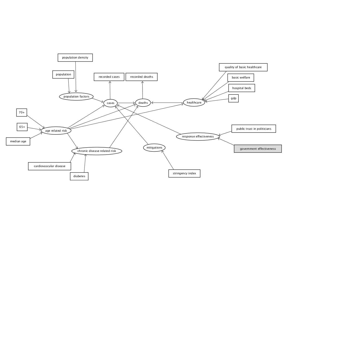
DAG
Data
library(tidyverse)
library(lavaan)
library(lubridate)
library(visdat)
library(dagitty)
library(janitor)
library(cowplot)
library(scales)
library(semPlot)
library(gfoRmula)
library(ggdag)
library(semTools)
library(data.table)
The datasets to be utilised are: * Our World in Data COVID Dataset (Our World in Data 2020) * Oxford Covid-19 Government Response Tracker (‘OxCGRT/covid-policy-tracker’ 2020) * Trust in Politicians from the Institutional Profiles Database(‘Institutional Profiles Database’ n.d.) * Government Effectiveness from Worldbank (‘WGI 2019 Interactive > Home’ n.d.) * Health equality and basic healthcare from GovData360 (‘GovData360: Health equality’ n.d.)
# COVID OWID
download.file("https://raw.githubusercontent.com/owid/covid-19-data/master/public/data/owid-covid-data.csv", "./data/covid_owid.csv")

# OxCGRT
download.file("https://github.com/OxCGRT/covid-policy-tracker/raw/master/data/OxCGRT_latest.csv", "./data/oxpol.csv")
# add inciremental weeks and months to the data
covid <- read.csv("./data/covid_owid.csv")
covid$month <- lubridate::month(covid$date, label = TRUE, abbr = TRUE)
covid$week <- lubridate::week(covid$date)
covid$week <- covid$week+1
covid[covid$week == 54, "week"] <- 1

#available data
names(covid)
##  [1] "iso_code"                        "continent"
##  [3] "location"                        "date"
##  [5] "total_cases"                     "new_cases"
##  [7] "total_deaths"                    "new_deaths"
##  [9] "total_cases_per_million"         "new_cases_per_million"
## [11] "total_deaths_per_million"        "new_deaths_per_million"
## [13] "total_tests"                     "new_tests"
## [15] "total_tests_per_thousand"        "new_tests_per_thousand"
## [17] "new_tests_smoothed"              "new_tests_smoothed_per_thousand"
## [19] "tests_units"                     "stringency_index"
## [21] "population"                      "population_density"
## [23] "median_age"                      "aged_65_older"
## [25] "aged_70_older"                   "gdp_per_capita"
## [27] "extreme_poverty"                 "cvd_death_rate"
## [29] "diabetes_prevalence"             "female_smokers"
## [31] "male_smokers"                    "handwashing_facilities"
## [33] "hospital_beds_per_thousand"      "life_expectancy"
## [35] "month"                           "week"
#visualise missing data
vis_dat(covid, warn_large_data = FALSE)
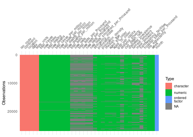
To reduce the noise in the variables the OWID dataset is summarised by week.
coviddata_sumweek <- covid %>%
  filter(location != "World", location != "International") %>%
  group_by(iso_code, week) %>%
  summarise(
            week_start = first(date),
            week_end = last(date),
            new_cases = sum(new_cases),
            new_deaths = sum(new_deaths),
            new_cases_per_million = sum(new_cases_per_million),
            new_deaths_per_million = sum(new_deaths_per_million),
            new_tests = sum(new_tests),
            new_tests_per_thousand = sum(new_tests_per_thousand),
            ) %>%
  ungroup()

join <- covid %>%
  select(-new_cases, -new_deaths, -new_cases_per_million, -new_deaths_per_million, -new_tests, -new_tests_per_thousand, -week) %>%
  mutate(week_end = date)

coviddata_sumweek<- merge(coviddata_sumweek, join, by = c("iso_code", "week_end"))
The additional metric datasets are imported and joined with the OWID dataset, the same method as in the previous project.
poltrustfull <- read_csv("./data/poltrustfull.csv")

poltrustfull <- poltrustfull %>%
  mutate(iso_code = country_iso3) %>%
  select(iso_code, x2018)
names(poltrustfull)[2] <- "trust_in_pol"

coviddata_m <- merge(coviddata_sumweek, poltrustfull, by = "iso_code")

#government effectiveness
gov_effect <- read_csv("./data/goveffect.csv")
gov_effect <- clean_names(gov_effect)
goveff <- gov_effect %>%
  filter(indicator == "Government Effectiveness", subindicator_type == "Estimate") %>%
  mutate(iso_code = country_iso3) %>%
  select(iso_code, x2018)
names(goveff)[2] <- "government_eff"

coviddata_m <- merge(coviddata_m, goveff, by = "iso_code")

glostatedemoc <- read_csv("./data/globalstatedemoc.csv")
glostatedemoc <- clean_names(glostatedemoc)

glostat_health <- glostatedemoc %>%
  filter(indicator == "Health equality" | indicator == "Basic welfare") %>%
  mutate(iso_code = country_iso3) %>%
  select(iso_code, indicator, x2018) %>%
  pivot_wider(names_from = indicator, values_from = x2018) %>%
  clean_names()

coviddata_m <- merge(coviddata_m, glostat_health, by = "iso_code")
Modelling
Structural equation modelling comes with a variety of challenges, the foremost is ensuring that the model is identified, there are a variety of tests to ensure a model is identified however the simplest method is to create a recursive model. A recursive model is directional, reflecting a DAG, as such the models used are all intended to be recursive models. (Thakkar 2020). A core challenge to this effort is that by measuring between countries, for non-time-varying models we are limited to a maximum of ~200 observations, this is very near the lower limit for data size for SEM, and for our initial model, below the suggested number of observations. As joining data from external sources was required, the number observations was further decreased reducing the chances of success and model convergence.
cvd_week5dplus <- coviddata_m %>%
  group_by(iso_code) %>%
  mutate(stringency_index = max(na.omit(stringency_index))) %>%
  ungroup() %>%
  filter(total_deaths >= 5) %>% #filter
  group_by(iso_code) %>%
  mutate(sincefive = row_number()) %>% #counting weeks
  filter(total_deaths == max(total_deaths)) %>%
  filter(date == min(date)) %>%
  ungroup() %>%
  filter(stringency_index > -1000, total_deaths > -1000)
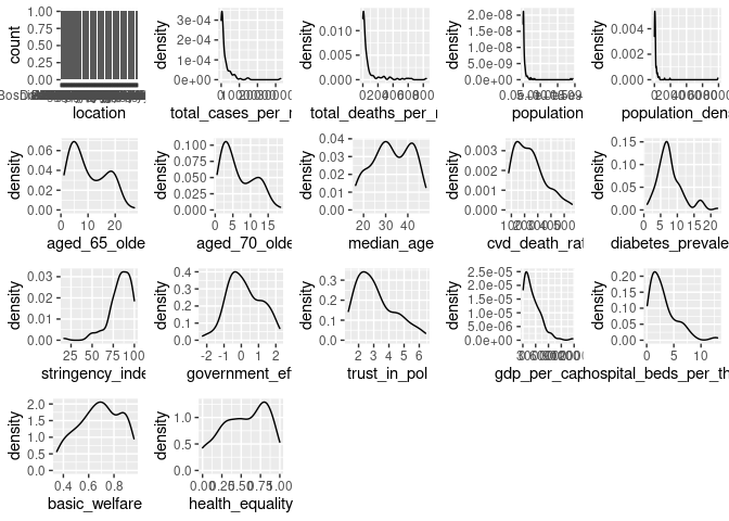
Data Checking
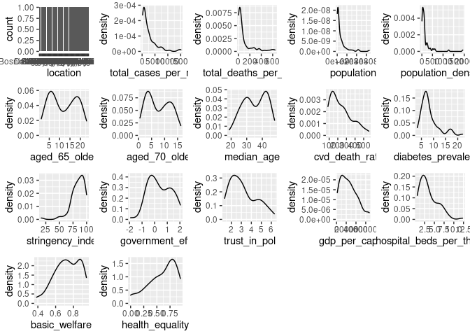
Originally SEM relied on all multivariate distributions being normal, where possible this is still recommended, however robust estimator methods have been developed to handle non-normal distributions.
# https://stackoverflow.com/questions/48507378/plotting-distributions-of-all-columns-in-an-r-data-frame
cvd_vars <- cvd_week5dplus %>%
  select(location, total_cases_per_million, total_deaths_per_million, population, population_density, aged_65_older, aged_70_older, median_age, cvd_death_rate, diabetes_prevalence, stringency_index, government_eff, trust_in_pol, gdp_per_capita, hospital_beds_per_thousand, basic_welfare, health_equality) %>%
  filter(stringency_index >= 0) %>%
  na.omit()


dist_plots <- lapply(names(cvd_vars), function(var_x){
  p <-
    ggplot(cvd_vars) +
    aes_string(var_x)

  if(is.numeric(cvd_vars[[var_x]])) {
    p <- p + geom_density()

  } else {
    p <- p + geom_bar()
  }

})

plot_grid(plotlist = dist_plots)
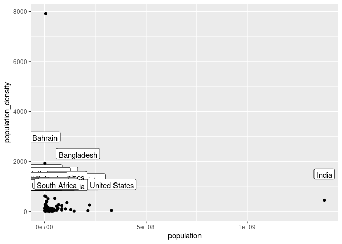
ggplot(cvd_vars, aes(x = total_cases_per_million, y = total_deaths_per_million)) + geom_point() + geom_label(aes(label = location))
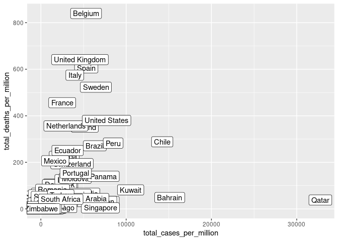
summary(cvd_vars$total_cases_per_million)
##     Min.  1st Qu.   Median     Mean  3rd Qu.     Max.
##     2.96   253.40   801.82  2231.46  2663.43 32770.23
summary(cvd_vars$total_deaths_per_million)
##    Min. 1st Qu.  Median    Mean 3rd Qu.    Max.
##   0.110   4.532  19.992  81.468  61.325 839.717
There is variation in distributions so a robust method must be selected. “MLR” is a recommended starting point if data quality is questionable. (Michael Hallquist 2018)
SEM is more effective when the data has had outliers removed, Belgium and Qatar represent outliers in cases and deaths per million respectively and have been removed. (Thakkar 2020). Similarly, Singapore, India and China have been removed due to their exceptionally high population.
cvd_vars <- cvd_vars %>%
  filter(location != "Belgium", location != "Qatar") %>%
  filter(total_cases_per_million >= 200, total_deaths_per_million >= 3)

ggplot(cvd_vars, aes(x = population, y = population_density)) + geom_point() + geom_label(aes(label = location), vjust = -2)
cvd_vars <- cvd_vars %>%
  filter(location != "Singapore", location != "India", location != "China")

dist_plots <- lapply(names(cvd_vars), function(var_x){
  p <-
    ggplot(cvd_vars) +
    aes_string(var_x)

  if(is.numeric(cvd_vars[[var_x]])) {
    p <- p + geom_density()

  } else {
    p <- p + geom_bar()
  }

})

plot_grid(plotlist = dist_plots)
summary(cvd_vars)
##    location         total_cases_per_million total_deaths_per_million
##  Length:80          Min.   :  202.3         Min.   :  3.377
##  Class :character   1st Qu.:  573.1         1st Qu.: 14.877
##  Mode  :character   Median : 1332.8         Median : 39.287
##                     Mean   : 2510.3         Mean   :101.883
##                     3rd Qu.: 2977.9         3rd Qu.:104.947
##                     Max.   :15106.5         Max.   :641.517
##    population        population_density aged_65_older    aged_70_older
##  Min.   :   875899   Min.   :   3.202   Min.   : 1.144   Min.   : 0.526
##  1st Qu.:  5342587   1st Qu.:  32.053   1st Qu.: 5.875   1st Qu.: 3.491
##  Median : 10566019   Median :  83.142   Median :11.143   Median : 7.157
##  Mean   : 35961743   Mean   : 160.602   Mean   :11.746   Mean   : 7.662
##  3rd Qu.: 43763080   3rd Qu.: 136.684   3rd Qu.:18.456   3rd Qu.:11.738
##  Max.   :331002647   Max.   :1935.907   Max.   :23.021   Max.   :16.240
##    median_age    cvd_death_rate   diabetes_prevalence stringency_index
##  Min.   :18.80   Min.   : 85.75   Min.   : 3.280      Min.   : 16.67
##  1st Qu.:29.25   1st Qu.:133.55   1st Qu.: 5.798      1st Qu.: 76.85
##  Median :35.50   Median :205.42   Median : 7.125      Median : 85.65
##  Mean   :35.18   Mean   :237.52   Mean   : 8.212      Mean   : 83.95
##  3rd Qu.:42.35   3rd Qu.:299.73   3rd Qu.: 9.328      3rd Qu.: 93.52
##  Max.   :47.90   Max.   :559.81   Max.   :22.020      Max.   :100.00
##  government_eff     trust_in_pol   gdp_per_capita  hospital_beds_per_thousand
##  Min.   :-1.9091   Min.   :1.324   Min.   : 1653   Min.   : 0.600
##  1st Qu.:-0.3416   1st Qu.:2.134   1st Qu.:11431   1st Qu.: 1.675
##  Median : 0.2977   Median :2.914   Median :23040   Median : 2.850
##  Mean   : 0.3915   Mean   :3.180   Mean   :25226   Mean   : 3.489
##  3rd Qu.: 1.1400   3rd Qu.:4.253   3rd Qu.:35975   3rd Qu.: 4.725
##  Max.   : 2.0396   Max.   :6.306   Max.   :67335   Max.   :12.270
##  basic_welfare    health_equality
##  Min.   :0.3857   Min.   :0.0000
##  1st Qu.:0.6403   1st Qu.:0.4605
##  Median :0.7425   Median :0.6579
##  Mean   :0.7288   Mean   :0.6000
##  3rd Qu.:0.8661   3rd Qu.:0.8026
##  Max.   :0.9464   Max.   :0.9474
Despite removing some outliers and a portion of the lowest values the distributions are still quite skewed for some statistics, the robust estimator functions may mitigate this in part. Additionally, the total number of observations has continued to decrease, however as this is the effort for evaluating the initial structure so we will proceed with the analysis.
Specify Structure
The DAG is now represented in Lavaan SEM format, latent variables represent the structure of our DAG and the data collected is used as measures of these latent variables.
init_model <- '
# latent variable model
pop_factors =~ population_density + population
age_risk =~ aged_65_older + aged_70_older + median_age
chronic_risk =~ cvd_death_rate + diabetes_prevalence
cases =~ total_cases_per_million
deaths =~ total_deaths_per_million
response_eff =~ trust_in_pol + government_eff + stringency_index
healthcare =~ basic_welfare + health_equality + hospital_beds_per_thousand


# regressions
cases ~ pop_factors + age_risk + response_eff
deaths ~ cases + age_risk + chronic_risk + healthcare

# covariance
chronic_risk ~~ age_risk
healthcare ~~ age_risk
aged_65_older ~~ aged_70_older
'
Lavaan produced and error and struggles to converge when variance between variables is large, as such the variables have been rescaled according to their distributions on a smaller scale.
cvd_vars <- cvd_vars %>%
  mutate_at(vars(-location), rescale, to = c(0,1))
When gradient check is active the model appears to have converged but there most variances and errors are NA, setting to false prevents some of this error.
cvd_sem <- sem(init_model, data = cvd_vars, estimator = "MLR", check.gradient = FALSE)
Negative variance is often a sign of an unidentified model, however as the model should be recursive this is unlikely to be the case, more likely is that the structure is too different from what the data represents and there is not possible solution, thus negative variances have to be introduced in order to enable fitting to occur, unfortunately negative variances indicate a failed model (Rosseel n.d.).
Research Evaluation
As is evident from the analysis of the DAGs and SEM the structure implied in the previous research was unlikely to produce a positive outcome and is unlikely to represent the observations available in the data. This is likely partly due to the choice to use countries for evaluation, and the large count of endogenous variables in this model represented by variables that are regressed by another variable. Further efforts to modify this structure are unlikely to be fruitful and not best practice (‘Best practices in SEM’ n.d.).
Build Up Approach and Confirmatory Factor Analysis (CFA)
A preferable alternative to the approach taken previously is to build up first a DAG, and then a model iterating informed by fit and variance (‘Best practices in SEM’ n.d.) to increase complexity and improve fit. An attempt at which is undertaken here. This attempt is still constrained by the data already collected but presents an opportunity to guide future investigation.
Simplified DAG
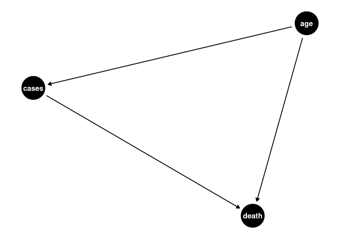
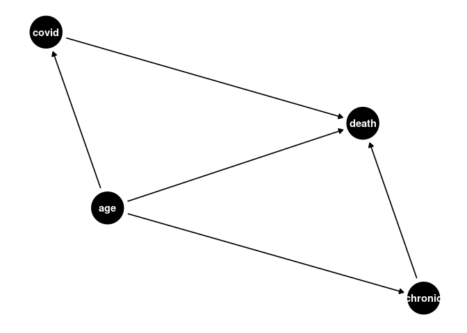
If we assume measurement error is not present, we can create a simple DAG for the effect of age, this DAG presents an opportunity for CFA, the measurement error is still somewhat accounted for by the SEM model.
a <- dagify(cases ~ age,
            death ~ age,
            death ~ cases)
ggdag(a) + theme_dag()
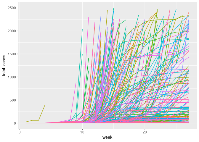
New Outcome Variable
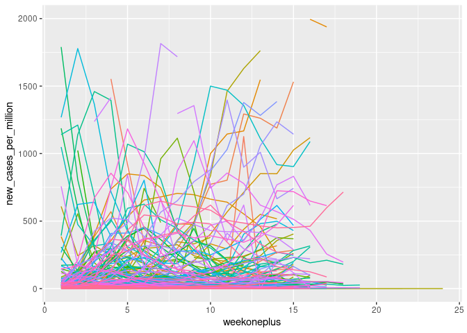
The previous research utilised total deaths and cumulative measures. Instead, the new outcome variable is created as the new_deaths_per_million, 4 weeks or 28 days after the first 100 cases. This allows the DAG to represent a non-time-varying snapshot of the pandemic. This allows time for gestation, and infection while also being on the upslope of many countries new case curves. Finally, to aid modelling the variance both new_cases_per_million and new_deaths_per_million will be log transformed.
covid_new <- covid %>%
  filter(location != "World", location != "International") %>%
  group_by(iso_code, week) %>%
  summarise(
            week_start = first(date),
            week_end = last(date),
            new_cases = sum(new_cases),
            new_deaths = sum(new_deaths),
            new_cases_per_million = sum(new_cases_per_million),
            new_deaths_per_million = sum(new_deaths_per_million),
            new_tests = sum(new_tests),
            new_tests_per_thousand = sum(new_tests_per_thousand),
            stringency_index = mean(stringency_index)
            ) %>%
  ungroup()

join <- covid %>%
  select(-new_cases, -new_deaths, -new_cases_per_million, -new_deaths_per_million, -new_tests, -new_tests_per_thousand, -week) %>%
  mutate(week_end = date, -stringency_index)

covid_new_m <- merge(covid_new, join, by = c("iso_code", "week_end"))
ggplot(covid_new_m, aes(x = week, y = total_cases, color = location)) + geom_line()+ theme(legend.position = "none") + ylim(0, 2500)
cvd_100c <- covid_new_m %>%
  group_by(iso_code) %>%
  filter(total_cases >= 100) %>%
  arrange(week) %>%
  mutate(weekoneplus = row_number()) %>%
  ungroup()

ggplot(cvd_100c, aes(x = weekoneplus, y = new_cases_per_million, color = location)) + geom_line()+ theme(legend.position = "none")+ ylim(0, 2000)
Log transformation of the variables induced unidentified values where they were zero which had to be rectified.
cvd_100c_p4 <- cvd_100c %>%
group_by(iso_code) %>%
filter(weekoneplus == 4) %>%
ungroup() %>%
mutate(logndpm = log(new_deaths_per_million), logncpm = log(new_cases_per_million))
cvd_100c_p4[cvd_100c_p4$logndpm < -1000, "logndpm"] <- 0
cvd_100c_p4[cvd_100c_p4$logncpm < -1000, "logncpm"] <- 0
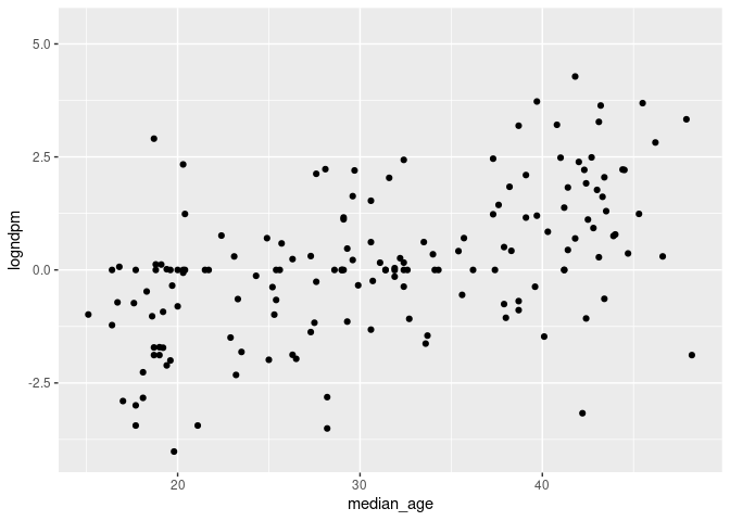
ggplot(cvd_100c_p4, aes(x = median_age, y = logndpm)) + geom_point()
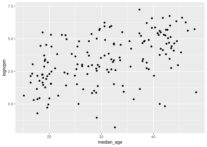
ggplot(cvd_100c_p4, aes(x = median_age, y = logncpm)) + geom_point()
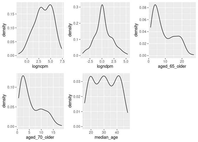
dist_plots <- lapply(list("logncpm", "logndpm", "aged_65_older", "aged_70_older", "median_age"), function(var_x){
  p <-
    ggplot(cvd_100c_p4) +
    aes_string(var_x)

  if(is.numeric(cvd_100c_p4[[var_x]])) {
    p <- p + geom_density()

  } else {
    p <- p + geom_bar()
  }

})

plot_grid(plotlist = dist_plots)
CFA Model
Model 1- Age, Cases, Deaths
Though cases is a much less reliable statistic than deaths due to measurement error differences in reporting and testing, etc (Our World in Data 2020), not including it in analysis leaves few other opportunities. As before, cases and deaths are latent variables of their measured outcomes which accounts for some of this error, age is a latent variable with three measures, median age of the country and proportions aged 65+ and aged 70+. Covariance between aged 65+ and aged 70+ is introduced due to their likely interaction.
cfa1_df <- cvd_100c_p4 %>%
mutate_at(vars(median_age, aged_65_older, aged_70_older, logncpm, logndpm), rescale, to = c(0,10))
cfa1_model <-'
# latent variables
age_risk =~ aged_70_older + median_age + aged_65_older
cases =~ logncpm
deaths =~ logndpm
# regressions (effects)
cases ~ age_risk
deaths ~ age_risk + cases
#covariances
aged_65_older ~~ aged_70_older
'
cfa1_sem <- cfa(cfa1_model, data = cfa1_df, estimator = "MLR")
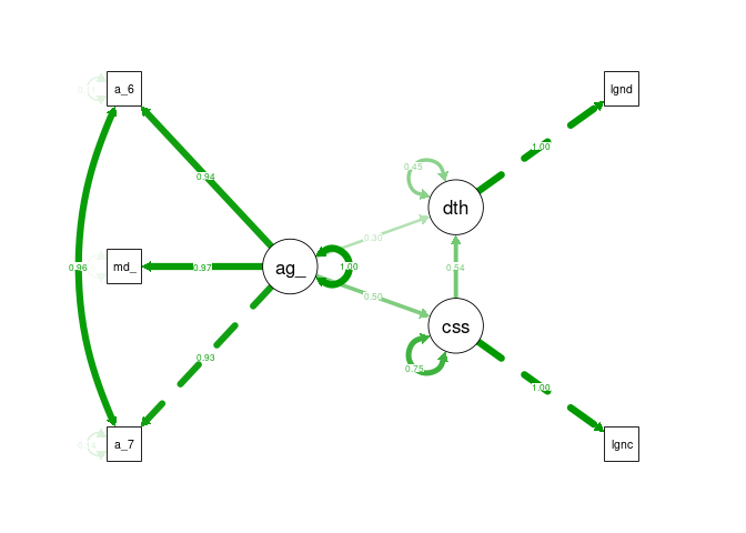
summary(cfa1_sem, fit.measures=TRUE, standardized=TRUE)
## lavaan 0.6-6 ended normally after 85 iterations
##
##   Estimator                                         ML
##   Optimization method                           NLMINB
##   Number of free parameters                         12
##
##                                                   Used       Total
##   Number of observations                           158         171
##
## Model Test User Model:
##                                                Standard      Robust
##   Test Statistic                                 11.759       9.965
##   Degrees of freedom                                  3           3
##   P-value (Chi-square)                            0.008       0.019
##   Scaling correction factor                                   1.180
##        Yuan-Bentler correction (Mplus variant)
##
## Model Test Baseline Model:
##
##   Test statistic                              1183.269     800.856
##   Degrees of freedom                                10          10
##   P-value                                        0.000       0.000
##   Scaling correction factor                                  1.478
##
## User Model versus Baseline Model:
##
##   Comparative Fit Index (CFI)                    0.993       0.991
##   Tucker-Lewis Index (TLI)                       0.975       0.971
##
##   Robust Comparative Fit Index (CFI)                         0.993
##   Robust Tucker-Lewis Index (TLI)                            0.977
##
## Loglikelihood and Information Criteria:
##
##   Loglikelihood user model (H0)              -1174.343   -1174.343
##   Scaling correction factor                                  1.221
##       for the MLR correction
##   Loglikelihood unrestricted model (H1)      -1168.463   -1168.463
##   Scaling correction factor                                  1.213
##       for the MLR correction
##
##   Akaike (AIC)                                2372.686    2372.686
##   Bayesian (BIC)                              2409.437    2409.437
##   Sample-size adjusted Bayesian (BIC)         2371.451    2371.451
##
## Root Mean Square Error of Approximation:
##
##   RMSEA                                          0.136       0.121
##   90 Percent confidence interval - lower         0.061       0.049
##   90 Percent confidence interval - upper         0.222       0.201
##   P-value RMSEA <= 0.05                          0.033       0.052
##
##   Robust RMSEA                                               0.132
##   90 Percent confidence interval - lower                     0.047
##   90 Percent confidence interval - upper                     0.226
##
## Standardized Root Mean Square Residual:
##
##   SRMR                                           0.011       0.011
##
## Parameter Estimates:
##
##   Standard errors                             Sandwich
##   Information bread                           Observed
##   Observed information based on                Hessian
##
## Latent Variables:
##                    Estimate  Std.Err  z-value  P(>|z|)   Std.lv  Std.all
##   age_risk =~
##     aged_70_older     1.000                               2.250    0.929
##     median_age        1.197    0.069   17.370    0.000    2.694    0.970
##     aged_65_older     1.025    0.012   88.324    0.000    2.305    0.942
##   cases =~
##     logncpm           1.000                               2.028    1.000
##   deaths =~
##     logndpm           1.000                               1.712    1.000
##
## Regressions:
##                    Estimate  Std.Err  z-value  P(>|z|)   Std.lv  Std.all
##   cases ~
##     age_risk          0.449    0.063    7.158    0.000    0.498    0.498
##   deaths ~
##     age_risk          0.227    0.054    4.239    0.000    0.299    0.299
##     cases             0.459    0.067    6.814    0.000    0.544    0.544
##
## Covariances:
##                    Estimate  Std.Err  z-value  P(>|z|)   Std.lv  Std.all
##  .aged_70_older ~~
##    .aged_65_older     0.704    0.327    2.152    0.031    0.704    0.961
##
## Variances:
##                    Estimate  Std.Err  z-value  P(>|z|)   Std.lv  Std.all
##    .aged_70_older     0.800    0.325    2.460    0.014    0.800    0.136
##    .median_age        0.453    0.364    1.245    0.213    0.453    0.059
##    .aged_65_older     0.670    0.329    2.035    0.042    0.670    0.112
##    .logncpm           0.000                               0.000    0.000
##    .logndpm           0.000                               0.000    0.000
##     age_risk          5.062    0.543    9.320    0.000    1.000    1.000
##    .cases             3.094    0.385    8.035    0.000    0.752    0.752
##    .deaths            1.326    0.140    9.485    0.000    0.452    0.452
This time modelling produced no errors and the fit measures are valid. The output is quite long but can be addressed in sections. It should be noted that measures are taken as their robust variants which are less effected by non-normal distributions (Savalei 2018).
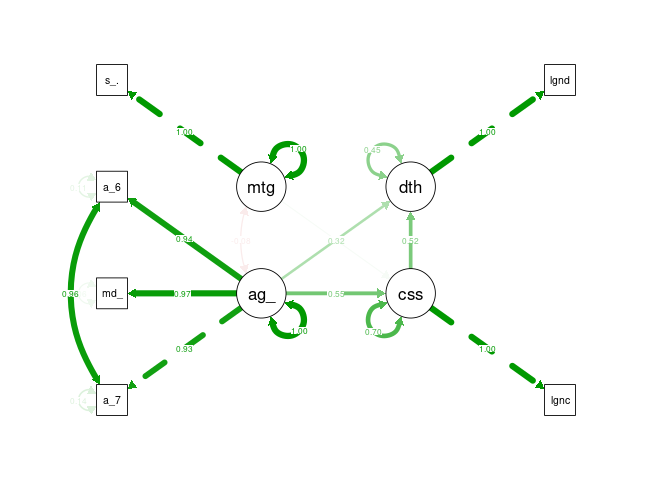
Fit SEM fit is a very loosely defined subject with many competing recommendations, Gana and Broc detail this and provide their own interpretation which will be the basis for model fit evaluation (Gana & Broc 2018). Chi Squared significance (CSS) and SRMR are suggested as the best indicator of absolute fit, the CSS value of 0.019 is below the 0.05 threshold indicating significance, unfortunately in SEM this indicates a poor fit. However, SRMR of 0.011 is well below the threshold suggested by G&B of 0.08 indicating a good fit. CFI and TLI indicate if the fit is better than the null model, for both indicators a value >0.95 indicates good fit. The model CFI 0.993 and TLI 0.977 are above this threshold indicating the model is a better fit than the null model. AIC and BIC are indicators of comparative fit between similar models, due to the large changes being undertaken between model iterations in this project are unlikely to be useful. Likelhood of RMSEA significance is low, the RMSEA itself is low, however so are the confidence interval bounds creating challenges in interpretation.
Overall, most fit indices indicate a good fit the DOF of the model is quite low and the sample quite small potentially contributing the issues with CSS values. The fit is not poor nor conclusive good either.
Coefficients and Variances The interpretation of coefficients and variances in SEM is more challenging due to the fixing of some variances and not other in the model, this behaviours can be modified but requires significant interrogation of the underlying causal structure for latent and total effects. For the above model, all variance estimates are reasonable within their ranges, age risk is quite high comparative to other variances but does not appear to be too unreasonable. Similarly, some of the free z-values are significant. This indicates there are no obvious errors within the model.
semPaths(cfa1_sem, what = "stand", rotation = 2, layout = "tree")
Model 2 - Age, Cases, Chronic Illness, Deaths
a <- dagify(covid ~ age,
            death ~ age,
            death ~ covid,
            chronic ~ age,
            death ~ chronic,
            exposure = "chronic",
            outcome = "death"
            )
ggdag(a) + theme_dag()
cfa2_df <- cvd_100c_p4 %>%
  mutate_at(vars(median_age, aged_65_older, aged_70_older, logncpm, logndpm, cvd_death_rate, diabetes_prevalence), rescale, to = c(0,10))

cfa2_model <-'
# latent variables
age_risk =~ aged_70_older + median_age + aged_65_older
cases =~ logncpm
deaths =~ logndpm
chronic_disease =~ cvd_death_rate + diabetes_prevalence

# regressions (effects)
cases ~ age_risk
deaths ~ age_risk + cases + chronic_disease


#covariances
aged_65_older ~~ aged_70_older
'

cfa2_sem <- cfa(cfa2_model, data = cfa2_df, estimator = "MLR")
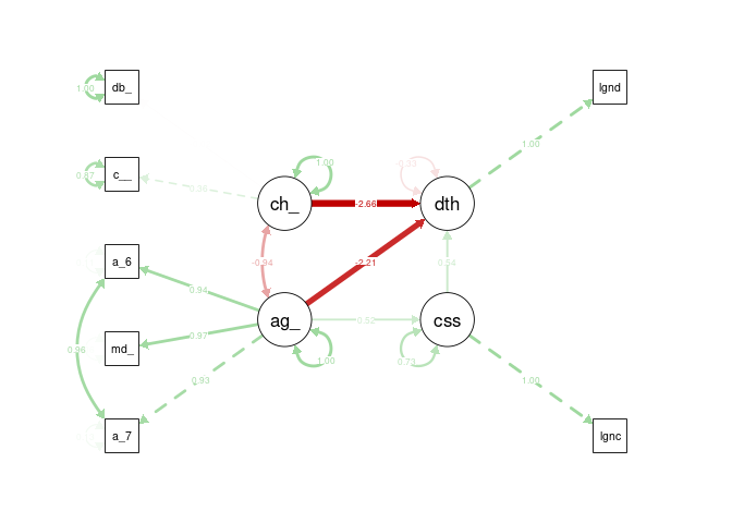
Despite many attempts to modify the structure and measures, incorporating chronic disease risk as a latent variable induced negative variances in the model, similar to the initial model. Therefore, this model is a failure.
semPaths(cfa2_sem, what = "stand", rotation = 2, layout = "tree")
CFA Model 3
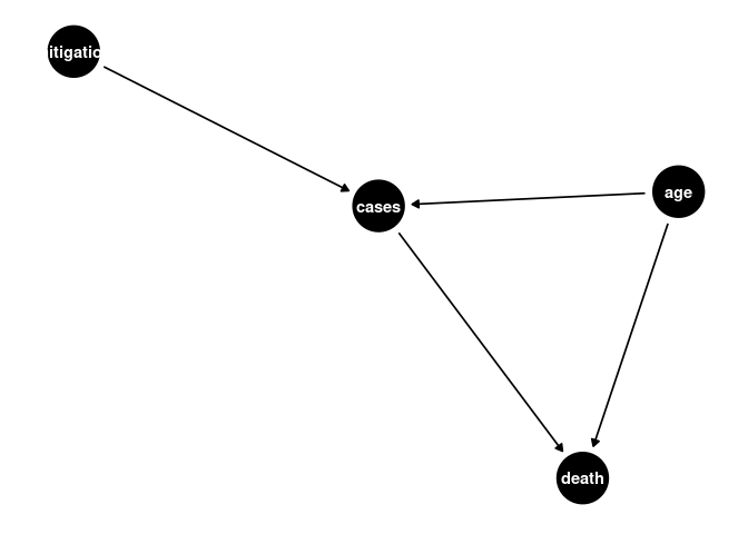
a <- dagify(cases ~ age,
            death ~ age,
            death ~ cases,
            cases ~ mitigation
            )
ggdag(a) + theme_dag()
cfa4_df <- cvd_100c_p4 %>%
  mutate_at(vars(median_age, aged_65_older, aged_70_older, logncpm, logndpm, cvd_death_rate, diabetes_prevalence, stringency_index.x), rescale, to = c(0,10))

cfa4_model <-'
# latent variables
age_risk =~ aged_70_older + median_age + aged_65_older
cases =~ logncpm
deaths =~ logndpm
mitigation =~ stringency_index.x

# regressions (effects)
cases ~ age_risk + mitigation
deaths ~ age_risk + cases

#covariances
aged_65_older ~~ aged_70_older
'

cfa4_sem <- cfa(cfa4_model, data = cfa4_df, estimator = "MLR")
summary(cfa4_sem, fit.measures=TRUE, standardized=TRUE)
## lavaan 0.6-6 ended normally after 95 iterations
##
##   Estimator                                         ML
##   Optimization method                           NLMINB
##   Number of free parameters                         15
##
##                                                   Used       Total
##   Number of observations                           146         171
##
## Model Test User Model:
##                                                Standard      Robust
##   Test Statistic                                 14.441      13.660
##   Degrees of freedom                                  6           6
##   P-value (Chi-square)                            0.025       0.034
##   Scaling correction factor                                   1.057
##        Yuan-Bentler correction (Mplus variant)
##
## Model Test Baseline Model:
##
##   Test statistic                              1117.732     859.202
##   Degrees of freedom                                15          15
##   P-value                                        0.000       0.000
##   Scaling correction factor                                  1.301
##
## User Model versus Baseline Model:
##
##   Comparative Fit Index (CFI)                    0.992       0.991
##   Tucker-Lewis Index (TLI)                       0.981       0.977
##
##   Robust Comparative Fit Index (CFI)                         0.993
##   Robust Tucker-Lewis Index (TLI)                            0.982
##
## Loglikelihood and Information Criteria:
##
##   Loglikelihood user model (H0)              -1372.645   -1372.645
##   Scaling correction factor                                  1.269
##       for the MLR correction
##   Loglikelihood unrestricted model (H1)      -1365.424   -1365.424
##   Scaling correction factor                                  1.209
##       for the MLR correction
##
##   Akaike (AIC)                                2775.289    2775.289
##   Bayesian (BIC)                              2820.043    2820.043
##   Sample-size adjusted Bayesian (BIC)         2772.577    2772.577
##
## Root Mean Square Error of Approximation:
##
##   RMSEA                                          0.098       0.094
##   90 Percent confidence interval - lower         0.032       0.027
##   90 Percent confidence interval - upper         0.164       0.158
##   P-value RMSEA <= 0.05                          0.097       0.114
##
##   Robust RMSEA                                               0.096
##   90 Percent confidence interval - lower                     0.025
##   90 Percent confidence interval - upper                     0.165
##
## Standardized Root Mean Square Residual:
##
##   SRMR                                           0.014       0.014
##
## Parameter Estimates:
##
##   Standard errors                             Sandwich
##   Information bread                           Observed
##   Observed information based on                Hessian
##
## Latent Variables:
##                    Estimate  Std.Err  z-value  P(>|z|)   Std.lv  Std.all
##   age_risk =~
##     aged_70_older     1.000                               2.285    0.930
##     median_age        1.183    0.069   17.238    0.000    2.702    0.968
##     aged_65_older     1.018    0.011   89.807    0.000    2.326    0.943
##   cases =~
##     logncpm           1.000                               2.034    1.000
##   deaths =~
##     logndpm           1.000                               1.725    1.000
##   mitigation =~
##     strngncy_ndx.x    1.000                               1.791    1.000
##
## Regressions:
##                    Estimate  Std.Err  z-value  P(>|z|)   Std.lv  Std.all
##   cases ~
##     age_risk          0.488    0.062    7.839    0.000    0.548    0.548
##     mitigation        0.040    0.084    0.475    0.635    0.035    0.035
##   deaths ~
##     age_risk          0.240    0.057    4.219    0.000    0.317    0.317
##     cases             0.439    0.073    6.051    0.000    0.517    0.517
##
## Covariances:
##                    Estimate  Std.Err  z-value  P(>|z|)   Std.lv  Std.all
##  .aged_70_older ~~
##    .aged_65_older     0.719    0.323    2.229    0.026    0.719    0.964
##   age_risk ~~
##     mitigation       -0.318    0.362   -0.877    0.380   -0.078   -0.078
##
## Variances:
##                    Estimate  Std.Err  z-value  P(>|z|)   Std.lv  Std.all
##    .aged_70_older     0.820    0.321    2.550    0.011    0.820    0.136
##    .median_age        0.484    0.343    1.411    0.158    0.484    0.062
##    .aged_65_older     0.678    0.324    2.091    0.037    0.678    0.111
##    .logncpm           0.000                               0.000    0.000
##    .logndpm           0.000                               0.000    0.000
##    .strngncy_ndx.x    0.000                               0.000    0.000
##     age_risk          5.220    0.584    8.939    0.000    1.000    1.000
##    .cases             2.900    0.399    7.266    0.000    0.701    0.701
##    .deaths            1.345    0.143    9.397    0.000    0.452    0.452
##     mitigation        3.208    0.588    5.455    0.000    1.000    1.000
All fit measures are improved over the initial simplified model, though chi-squared is still within the significant range. This model is a better fit than the previous model overall, though still unlikely objectively good fit.
semPaths(cfa4_sem, what = "stand", rotation = 2, layout = "tree")
Static Statistics Attempts were made to substitute in additional static statistics such as government effectiveness and healthcare however this often resulted in model errors or poorer fit.
Time Varying Model
The previous model while still not showing a good fit overall does indicate that there is an improvement in fit when including mitigation factors. The previous DAG is quite unrealistic however as the relationship between these variables is time varying, as cases initially drove stringency, and then stringency effects subsequent case numbers. Developing a time-varying model induces significant bias that is difficult to overcome, requiring g-methods (Hernán & Robins n.d.), but may improve understanding of the structure.
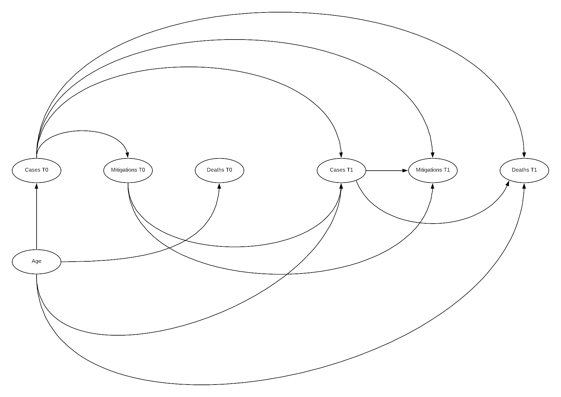
DAG
Here the DAG illustrates why time varying models are so challenging to manage systematic bias within. Additionally, as outlined by Hernan, there is often time-varying measurement error in such a model increasing complexity, this has not been included here (Hernán & Robins n.d.). The above DAG illustrates the relationship between an initial state 0, and a subsequent state 1, this can be repeated n times. Below this state 0 is the state we have been utilising previously, and state 1 is an additional 4 weeks after state 0.
cvd_100c_p8 <- cvd_100c %>%
  filter(iso_code != "ECU", weekoneplus == 8) %>%
  mutate(logndpm = log(new_deaths_per_million), logncpm = log(new_cases_per_million))

cvd_100c_p8[cvd_100c_p8$logndpm < -1000, "logndpm"] <- 0
cvd_100c_p8[cvd_100c_p8$logncpm < -1000, "logncpm"] <- 0

timevar <- merge(cvd_100c_p4, cvd_100c_p8, by = "iso_code")
cfa_tv <- timevar %>%
  mutate_at(vars(median_age.x, aged_65_older.x, aged_70_older.x, logncpm.x, logndpm.x, stringency_index.x.x,
                 median_age.y, aged_65_older.y, aged_70_older.y, logncpm.y, logndpm.y, stringency_index.x.y), rescale, to = c(0,10))

cfa_tv_model <-'
# latent variables
age_risk =~ aged_70_older.x + median_age.x + aged_65_older.x
cases0 =~ logncpm.x
cases1 =~ logncpm.y
deaths0 =~ logndpm.x
deaths1 =~ logndpm.y
mitigation0 =~ stringency_index.x.x
mitigation1 =~ stringency_index.x.y

# regressions (effects)

deaths1 ~ age_risk + cases1 + cases0
mitigation1 ~ cases0 + cases1 + mitigation0
cases1 ~ age_risk + mitigation0 + cases0
deaths0 ~ age_risk + cases0
mitigation0 ~ cases0
cases0 ~ age_risk

#covariances
aged_65_older.x ~~ aged_70_older.x
'

cfa_tv_sem <- sem(cfa_tv_model, data = cfa_tv, estimator = "MLR")
summary(cfa_tv_sem, fit.measures=TRUE, standardized=TRUE)
## lavaan 0.6-6 ended normally after 88 iterations
##
##   Estimator                                         ML
##   Optimization method                           NLMINB
##   Number of free parameters                         29
##
##                                                   Used       Total
##   Number of observations                           124         158
##
## Model Test User Model:
##                                                Standard      Robust
##   Test Statistic                                 33.106      28.620
##   Degrees of freedom                                 16          16
##   P-value (Chi-square)                            0.007       0.027
##   Scaling correction factor                                   1.157
##        Yuan-Bentler correction (Mplus variant)
##
## Model Test Baseline Model:
##
##   Test statistic                              1333.723     978.237
##   Degrees of freedom                                36          36
##   P-value                                        0.000       0.000
##   Scaling correction factor                                  1.363
##
## User Model versus Baseline Model:
##
##   Comparative Fit Index (CFI)                    0.987       0.987
##   Tucker-Lewis Index (TLI)                       0.970       0.970
##
##   Robust Comparative Fit Index (CFI)                         0.989
##   Robust Tucker-Lewis Index (TLI)                            0.974
##
## Loglikelihood and Information Criteria:
##
##   Loglikelihood user model (H0)              -1769.517   -1769.517
##   Scaling correction factor                                  1.386
##       for the MLR correction
##   Loglikelihood unrestricted model (H1)      -1752.963   -1752.963
##   Scaling correction factor                                  1.305
##       for the MLR correction
##
##   Akaike (AIC)                                3597.033    3597.033
##   Bayesian (BIC)                              3678.821    3678.821
##   Sample-size adjusted Bayesian (BIC)         3587.122    3587.122
##
## Root Mean Square Error of Approximation:
##
##   RMSEA                                          0.093       0.080
##   90 Percent confidence interval - lower         0.047       0.032
##   90 Percent confidence interval - upper         0.138       0.123
##   P-value RMSEA <= 0.05                          0.060       0.129
##
##   Robust RMSEA                                               0.086
##   90 Percent confidence interval - lower                     0.029
##   90 Percent confidence interval - upper                     0.136
##
## Standardized Root Mean Square Residual:
##
##   SRMR                                           0.065       0.065
##
## Parameter Estimates:
##
##   Standard errors                             Sandwich
##   Information bread                           Observed
##   Observed information based on                Hessian
##
## Latent Variables:
##                    Estimate  Std.Err  z-value  P(>|z|)   Std.lv  Std.all
##   age_risk =~
##     aged_70_oldr.x    1.000                               2.319    0.928
##     median_age.x      1.117    0.064   17.508    0.000    2.590    0.964
##     aged_65_oldr.x    1.013    0.012   86.402    0.000    2.349    0.942
##   cases0 =~
##     logncpm.x         1.000                               2.102    1.000
##   cases1 =~
##     logncpm.y         1.000                               1.989    1.000
##   deaths0 =~
##     logndpm.x         1.000                               1.766    1.000
##   deaths1 =~
##     logndpm.y         1.000                               2.237    1.000
##   mitigation0 =~
##     strngncy_ndx..    1.000                               1.778    1.000
##   mitigation1 =~
##     strngncy_ndx..    1.000                               1.748    1.000
##
## Regressions:
##                    Estimate  Std.Err  z-value  P(>|z|)   Std.lv  Std.all
##   deaths1 ~
##     age_risk          0.376    0.104    3.603    0.000    0.390    0.390
##     cases1            0.595    0.109    5.462    0.000    0.529    0.529
##     cases0            0.038    0.152    0.249    0.803    0.036    0.036
##   mitigation1 ~
##     cases0           -0.010    0.076   -0.126    0.900   -0.012   -0.012
##     cases1            0.172    0.107    1.614    0.107    0.196    0.196
##     mitigation0       0.731    0.091    8.052    0.000    0.743    0.743
##   cases1 ~
##     age_risk         -0.253    0.069   -3.684    0.000   -0.295   -0.295
##     mitigation0      -0.063    0.080   -0.789    0.430   -0.056   -0.056
##     cases0            0.857    0.079   10.911    0.000    0.906    0.906
##   deaths0 ~
##     age_risk          0.268    0.063    4.242    0.000    0.351    0.351
##     cases0            0.418    0.078    5.340    0.000    0.497    0.497
##   mitigation0 ~
##     cases0           -0.061    0.083   -0.736    0.462   -0.072   -0.072
##   cases0 ~
##     age_risk          0.524    0.066    7.926    0.000    0.578    0.578
##
## Covariances:
##                      Estimate  Std.Err  z-value  P(>|z|)   Std.lv  Std.all
##  .aged_70_older.x ~~
##    .aged_65_oldr.x      0.753    0.317    2.377    0.017    0.753    0.962
##  .deaths0 ~~
##    .deaths1             0.951    0.188    5.065    0.000    0.563    0.563
##    .mitigation1        -0.103    0.116   -0.891    0.373   -0.077   -0.077
##  .deaths1 ~~
##    .mitigation1        -0.276    0.197   -1.401    0.161   -0.162   -0.162
##
## Variances:
##                    Estimate  Std.Err  z-value  P(>|z|)   Std.lv  Std.all
##    .aged_70_oldr.x    0.866    0.322    2.693    0.007    0.866    0.139
##    .median_age.x      0.509    0.313    1.623    0.104    0.509    0.071
##    .aged_65_oldr.x    0.706    0.313    2.258    0.024    0.706    0.114
##    .logncpm.x         0.000                               0.000    0.000
##    .logncpm.y         0.000                               0.000    0.000
##    .logndpm.x         0.000                               0.000    0.000
##    .logndpm.y         0.000                               0.000    0.000
##    .strngncy_ndx..    0.000                               0.000    0.000
##    .strngncy_ndx..    0.000                               0.000    0.000
##     age_risk          5.375    0.527   10.195    0.000    1.000    1.000
##    .cases0            2.940    0.446    6.588    0.000    0.665    0.665
##    .cases1            1.553    0.222    7.001    0.000    0.393    0.393
##    .deaths0           1.333    0.165    8.095    0.000    0.427    0.427
##    .deaths1           2.140    0.295    7.243    0.000    0.428    0.428
##    .mitigation0       3.144    0.624    5.041    0.000    0.995    0.995
##    .mitigation1       1.354    0.320    4.232    0.000    0.443    0.443
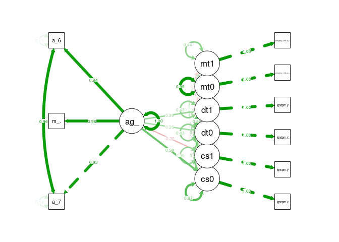
Somewhat surprisingly, there were no errors in processing the model. Unfortunately, model fit indicators are performing poorer, CSS is decreased and SRMR has increased above the 0.05 threshold. Comparative fit indices are reduced, though RMSEA is also reduced which is positive. A worthwhile test, but unfortunately not fully successful.
semPaths(cfa_tv_sem, what = "stand", rotation = 2, layout = "tree")
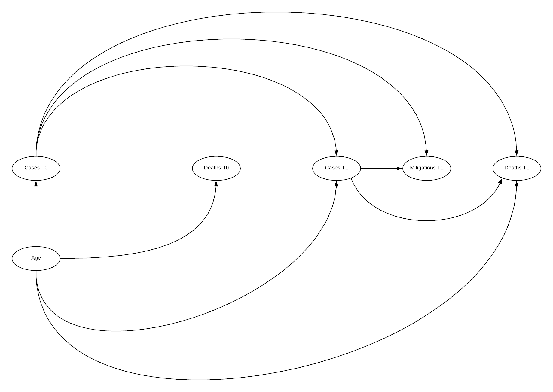
DAG
cfa_tv_model <-'
# latent variables
age_risk =~ aged_70_older.x + median_age.x + aged_65_older.x
cases0 =~ logncpm.x
cases1 =~ logncpm.y
deaths0 =~ logndpm.x
deaths1 =~ logndpm.y
mitigation1 =~ stringency_index.x.y

# regressions (effects)

deaths1 ~ age_risk + cases1 + cases0
mitigation1 ~ cases0 + cases1
cases1 ~ age_risk  + cases0
deaths0 ~ age_risk + cases0
cases0 ~ age_risk

#covariances
aged_65_older.x ~~ aged_70_older.x
'

cfa_tv_sem <- sem(cfa_tv_model, data = cfa_tv, estimator = "MLR")
summary(cfa_tv_sem, fit.measures=TRUE, standardized=TRUE)
## lavaan 0.6-6 ended normally after 90 iterations
##
##   Estimator                                         ML
##   Optimization method                           NLMINB
##   Number of free parameters                         25
##
##                                                   Used       Total
##   Number of observations                           124         158
##
## Model Test User Model:
##                                                Standard      Robust
##   Test Statistic                                 20.495      17.991
##   Degrees of freedom                                 11          11
##   P-value (Chi-square)                            0.039       0.082
##   Scaling correction factor                                   1.139
##        Yuan-Bentler correction (Mplus variant)
##
## Model Test Baseline Model:
##
##   Test statistic                              1218.338     919.909
##   Degrees of freedom                                28          28
##   P-value                                        0.000       0.000
##   Scaling correction factor                                  1.324
##
## User Model versus Baseline Model:
##
##   Comparative Fit Index (CFI)                    0.992       0.992
##   Tucker-Lewis Index (TLI)                       0.980       0.980
##
##   Robust Comparative Fit Index (CFI)                         0.993
##   Robust Tucker-Lewis Index (TLI)                            0.983
##
## Loglikelihood and Information Criteria:
##
##   Loglikelihood user model (H0)              -1573.616   -1573.616
##   Scaling correction factor                                  1.267
##       for the MLR correction
##   Loglikelihood unrestricted model (H1)      -1563.369   -1563.369
##   Scaling correction factor                                  1.228
##       for the MLR correction
##
##   Akaike (AIC)                                3197.232    3197.232
##   Bayesian (BIC)                              3267.739    3267.739
##   Sample-size adjusted Bayesian (BIC)         3188.688    3188.688
##
## Root Mean Square Error of Approximation:
##
##   RMSEA                                          0.083       0.072
##   90 Percent confidence interval - lower         0.018       0.000
##   90 Percent confidence interval - upper         0.139       0.126
##   P-value RMSEA <= 0.05                          0.150       0.237
##
##   Robust RMSEA                                               0.076
##   90 Percent confidence interval - lower                     0.000
##   90 Percent confidence interval - upper                     0.138
##
## Standardized Root Mean Square Residual:
##
##   SRMR                                           0.036       0.036
##
## Parameter Estimates:
##
##   Standard errors                             Sandwich
##   Information bread                           Observed
##   Observed information based on                Hessian
##
## Latent Variables:
##                    Estimate  Std.Err  z-value  P(>|z|)   Std.lv  Std.all
##   age_risk =~
##     aged_70_oldr.x    1.000                               2.321    0.929
##     median_age.x      1.115    0.066   16.983    0.000    2.587    0.963
##     aged_65_oldr.x    1.013    0.012   86.612    0.000    2.351    0.942
##   cases0 =~
##     logncpm.x         1.000                               2.102    1.000
##   cases1 =~
##     logncpm.y         1.000                               1.982    1.000
##   deaths0 =~
##     logndpm.x         1.000                               1.763    1.000
##   deaths1 =~
##     logndpm.y         1.000                               2.230    1.000
##   mitigation1 =~
##     strngncy_ndx..    1.000                               1.752    1.000
##
## Regressions:
##                    Estimate  Std.Err  z-value  P(>|z|)   Std.lv  Std.all
##   deaths1 ~
##     age_risk          0.354    0.107    3.320    0.001    0.369    0.369
##     cases1            0.586    0.110    5.314    0.000    0.521    0.521
##     cases0            0.058    0.153    0.376    0.707    0.054    0.054
##   mitigation1 ~
##     cases0           -0.061    0.105   -0.583    0.560   -0.074   -0.074
##     cases1            0.182    0.115    1.582    0.114    0.206    0.206
##   cases1 ~
##     age_risk         -0.237    0.074   -3.214    0.001   -0.277   -0.277
##     cases0            0.850    0.080   10.684    0.000    0.902    0.902
##   deaths0 ~
##     age_risk          0.261    0.063    4.112    0.000    0.344    0.344
##     cases0            0.422    0.079    5.369    0.000    0.503    0.503
##   cases0 ~
##     age_risk          0.524    0.066    7.911    0.000    0.578    0.578
##
## Covariances:
##                      Estimate  Std.Err  z-value  P(>|z|)   Std.lv  Std.all
##  .aged_70_older.x ~~
##    .aged_65_oldr.x      0.742    0.334    2.219    0.027    0.742    0.962
##  .deaths0 ~~
##    .deaths1             0.951    0.187    5.072    0.000    0.563    0.563
##    .mitigation1        -0.025    0.166   -0.150    0.880   -0.012   -0.012
##  .deaths1 ~~
##    .mitigation1        -0.117    0.254   -0.461    0.645   -0.046   -0.046
##
## Variances:
##                    Estimate  Std.Err  z-value  P(>|z|)   Std.lv  Std.all
##    .aged_70_oldr.x    0.855    0.339    2.523    0.012    0.855    0.137
##    .median_age.x      0.520    0.329    1.580    0.114    0.520    0.072
##    .aged_65_oldr.x    0.696    0.331    2.104    0.035    0.696    0.112
##    .logncpm.x         0.000                               0.000    0.000
##    .logncpm.y         0.000                               0.000    0.000
##    .logndpm.x         0.000                               0.000    0.000
##    .logndpm.y         0.000                               0.000    0.000
##    .strngncy_ndx..    0.000                               0.000    0.000
##     age_risk          5.386    0.528   10.201    0.000    1.000    1.000
##    .cases0            2.941    0.446    6.594    0.000    0.666    0.666
##    .cases1            1.567    0.224    6.991    0.000    0.399    0.399
##    .deaths0           1.332    0.165    8.091    0.000    0.429    0.429
##    .deaths1           2.140    0.295    7.248    0.000    0.430    0.430
##    .mitigation1       2.992    0.605    4.943    0.000    0.975    0.975
The above model indicates good fit across all fit indices! Chi-squared has moved above the significant threshold, though still low, SRMR increased though is still below the threshold. CFI and TLI are both improved, similarly across all RMSE indicators. The paths visualisation is similar to previous visualisations. There are some suggested improvements in the model, however disconnecting mitigations 1 from cases 0 is unlikely to be represented of the true causal path.
reliability(cfa_tv_sem)
##     alpha     omega    omega2    omega3    avevar
## 0.9748320 0.9367829 0.9367829 0.9374871 0.8947247
All reliability scores are above the threshold.
resid(cfa_tv_sem, "cor")
## $type
## [1] "cor.bollen"
##
## $cov
##                      a_70_. mdn_g. a_65_. lgncpm.x lgncpm.y lgndpm.x lgndpm.y
## aged_70_older.x       0.000
## median_age.x         -0.002  0.000
## aged_65_older.x       0.000 -0.001  0.000
## logncpm.x             0.008  0.018 -0.011  0.000
## logncpm.y             0.006  0.021 -0.013  0.000    0.000
## logndpm.x             0.021 -0.001  0.011  0.000   -0.023    0.000
## logndpm.y             0.034  0.002  0.021  0.004   -0.009   -0.007    0.000
## stringency_index.x.y -0.129 -0.054 -0.140  0.000    0.000   -0.035   -0.035
##                      str_..
## aged_70_older.x
## median_age.x
## aged_65_older.x
## logncpm.x
## logncpm.y
## logndpm.x
## logndpm.y
## stringency_index.x.y  0.000
There appears to be no highly significant difference between observed and implied correlations, stringency sitting just above threshold values, though the statistics indicate the model tends over predict correlation resulting in mostly negative values (Michael Hallquist 2018).
Overall indications are that a time varying model is the most accurate, particularly when there is a zero state present where no mitigation was taken, this could potentially relate to a need to lead and lag some variables. Hernan suggests that in order to undertake investigation into time varying causal models, g-methods must be implemented. (Hernán & Robins n.d.)
G-methods
Attempts were made to incorporate g-methods based on counterfactual consistency and inverse weighting (Naimi, Cole & Kennedy 2016) as described by Hernan, using the gfoRmula package (Lin et al. 2019) however, these methods require a much deeper understanding of statistics, expert knowledge of the subject matter and best practice. The referenced paper (Naimi, Cole & Kennedy 2016) opens that uptake by professional epidemiologists was hampered by the complexities understanding concepts and technical details.
First the structure of the data needs to be modified into the format ID, time index, covariates, treatment, outcome. For the analysis this will be, iso_code, weekoneplus, covariates (log of new cases per million, median age), stringency index, log of new deaths per million.
 cvd_g <- cvd_100c %>%
  mutate(weekoneplus = weekoneplus -1) %>%
  filter(iso_code != "ECU", iso_code != "UGA", iso_code != "BEN",
         iso_code != "CTU", iso_code != "FIN", iso_code != "ESP", iso_code != "LTU") %>%
  mutate(logndpm = log(new_deaths_per_million), logncpm = log(new_cases_per_million)) %>%
  mutate_at(vars(median_age, aged_65_older, aged_70_older, logncpm, logndpm, stringency_index.x), rescale, to = c(0,10)) %>%
  select(iso_code, weekoneplus, median_age, logncpm, logndpm, stringency_index.x) %>%
  na.omit()

cvd_g[cvd_g$logndpm < -1000, "logndpm"] <- 0
cvd_g[cvd_g$logncpm < -1000, "logncpm"] <- 0

cvd_g$iso_code <- as.factor(cvd_g$iso_code)
cvd_g_n <- cvd_g
cvd_g_n$iso_code <- as.numeric(cvd_g_n$iso_code)

gmethdf <- cvd_g_n %>%
  filter(weekoneplus <= 5) %>%
  mutate(weekoneplus = weekoneplus -1) %>%
  filter(iso_code != 10, iso_code != 42, iso_code != 3, iso_code != 124, iso_code != 148, iso_code != 78, iso_code != 90, iso_code != 92, iso_code != 96, iso_code != 129)
Transformation complete now into model structure. (Lin et al. 2019)
gformula_continuous_eof(obs_data = gmethdf,
                        id = "iso_code",
                        time_name = "weekoneplus",
                        outcome_name = "logndpm",
                        covnames = c("logncpm", "stringency_index.x"),
                        basecovs = "median_age",
                        covtypes = c("normal", "normal"),
                        histories = c(lagged),
                        histvars = list(c("logncpm", "stringency_index.x")),
                        covparams = list(covmodels = c(
                          logncpm ~ lag1_logncpm + lag1_stringency_index.x + weekoneplus,
                          stringency_index.x ~ lag1_logncpm + weekoneplus
                        )),
                        ymodel = logndpm ~ median_age + logncpm + lag1_logncpm + stringency_index.x + lag1_stringency_index.x,
                        seed = 222
                        )
Unfortunately I could not trouble shoot the error “Error in int_result/ref_mean : non-numeric argument to binary operator” despite numerous modifications. Further work will be required to implement this model type.
Outcomes
Conclusions
It is evident from the analysis in Appendix B that the structure and casual pathways implied by the previous research effort (Danny Lei Han et al. 2020) induced many opportunities for systemic bias and few attempts to mitigate these. The inability to model the implied DAG in SEM aids to verify this assumption that it is unlikely the inferred casual pathways were reflected in the observational data. Later efforts to develop a model that could aid in developing future research efforts were necessarily quite simplified structures. Most efforts met with minimal success with a mix of good and poor fit indications. The final time varied effort revealed a potential causal structure that is reflected in the observational data, however while most indices indicated good fit, most were still close to acceptable threshold values. Unfortunately modelling utilising g-methods methods was unsuccessful, however this approach is a potential candidate for evaluating a full time varied model effectively.
Reflection
The deeper I dove into Structural Equation Modelling and Causal Inference the more I realised the topic of COVID-19 is far too complex and the data too incomplete or poorly recorded for the application of these methods to be truly effective. While these methods are requirements to understanding the pandemic, due particularly to the large amount of observational data available, their application by an amateur and with limited data is unlikely to see any positive outcomes.
That said, of the available methods these were by far the most interesting to me, I chose to peruse this method based on that interest. The method opens understanding into not only new statistical methods as observed in other methods, but frameworks for identifying, communicating and assessing complex problems utilising DAGs and causal inference, topics which I will continue to investigate. To this end I kept on digging my hole deeper, I have learnt a great deal however the outcomes could have been improved. I believe including other areas of statics would have potentially improved overall outcomes on reflection, particularly looking into time series and accurately interpret lead and lag of variables, or potentially create a multi-level SEM model.
Overall, I’m glad I chose this method for the learning opportunities I gained, achieving a just passable fit on the complex time varied model was enough of an achievement. As long as I interpreted the outcomes correctly. # References
‘Best practices in SEM’ n.d.
Danny Lei Han, Emma Valme, Hemendra Patil, Joshua McCarthy, Lhalid Almundayfir & Leon MA 2020, COVID19_COVIDResearch_20200727.Pdf.
Gana, K. & Broc, G. 2018, Structural Equation Modeling with lavaan, John Wiley & Sons, Inc., Hoboken, NJ, USA.
‘GovData360: Health equality’ n.d., GovData360.
HarvardX PH559x 2020, Causal Diagrams: Draw Your Assumptions Before Your Conclusions.
Hernán, M.A. & Robins, J.M. n.d., Causal Inference: What If, p. 311.
‘How would I set up second order factors (hierarchical models) for confirmatory factor analysis in the R package ’lavaan’?’ n.d., ResearchGate.
‘Institutional Profiles Database’ n.d.
Lin, V., McGrath, S., Zhang, Z., Petito, L.C., Logan, R.W., Hernán, M.A. & Young, J.G. 2019, ‘gfoRmula: An R package for estimating effects of general time-varying treatment interventions via the parametric g-formula’, arXiv:1908.07072 [stat].
Michael Hallquist 2018, Introductory SEM using lavaan.
Naimi, A.I., Cole, S.R. & Kennedy, E.H. 2016, ‘An Introduction to G Methods’, International Journal of Epidemiology, p. dyw323.
Our World in Data 2020, ‘Owid/covid-19-data’, GitHub.
‘OxCGRT/covid-policy-tracker’ 2020.
Rosseel, Y. n.d., Structural Equation Modeling with lavaan, p. 127.
Savalei, V. 2018, ‘On the Computation of the RMSEA and CFI from the Mean-And-Variance Corrected Test Statistic with Nonnormal Data in SEM’, Multivariate Behavioral Research, vol. 53, no. 3, pp. 419–29.
Thakkar, J.J. 2020, Structural Equation Modelling: Application for Research and Practice (with AMOS and R), Studies in Systems, Decision and Control, vol. 285, Springer Singapore, Singapore.
‘WGI 2019 Interactive > Home’ n.d.
Apendicies
Appendix A
Appendix A
Implied Structure Repeated instances of the same implication in a different section are not repeated. The implications measured and or posited through analysis are highlighted in bold
Introduction
- Total cases per million population varied between locations due to measured and unmeasured factors
- Extremely small population countries had very high case/population due to their low population
- Total deaths per million population is less dependent on cases/population than other factors
- Extremely small population countries had very high deaths/population due to their low population
- The responses a countries government makes in response to covid are causes for variation between cases and deaths per population
- More responses indicate a “better” response
Country Based Age Influence
- Age distribution between countries is a result of many unobserved factors
- Age of a population effects the outcomes during pandemic’s epidemics and emergencies such as COVID-19
- Conditioning age to higher values is associated with poorer COVID-19 outcomes
- Variation in COVID-19 outcomes is not only associated with age
- The total deaths are associated with an increased time since initial COVID-19 infections
- Industrialized nations are associated with a higher median age
- Richer countries may be associated with a higher median age. (We can take richer here to mean GDP per capita)
- Recording of death due to COVID may be subject to error
- Methods of classifying deaths due to covid may have contributed to causing that error
- Conditioning on age does not rule out associations between increased risk and other factors
Patient Case Based Analysis
- Being the first country exposed to COVID is associated with comprehensive data collection
- Disclosure of information varies between countries
- Is there an association between COVID symptoms and chronic diseases
- Is increased age associated with chronic disease
- Is increased age associated with weakened immune system and therefore more susceptible to COVID
- Conditioning reproduction number to 1 is causally associated with disease spread (transmission)
- Conditioning on reproduction number 0 is associated with and end of transmission 24 High reproduction rate causes increase in pharmaceutical (medical) interventions
- Medical interventions are associated with reduced transmission
- Symptom onset is associated with time since infection
- Longer time periods between exposure and onset of symptoms is a cause of transmission
- Identification of symptoms for COVID is associated with identification of symptoms for the flu
- COVID patients with poor outcomes is caused by the immune system attacking healthy cells (immune disorder)
- Immune disorder is associated with infection
- Immune disorder is associated with organ failure
- Mean of age distribution is associated with true age
- Conditioning location to the United States is associated with higher age
- Conditioning location the United States is associated with a lower rate of infection at lower ages
- Conditioning location to the United States is associated with increased cases
- Symptoms are associated with chronic disease
- Symptoms are associated with COVID
- COVID diagnosis is negatively associated with the presence of symptoms due to chronic disease
Conditioning for individuals with COVID; 39. Conditioning symptoms to pneumonia is associated with chronic disease 39. Conditioning symptoms to acute respiratory is associated with chronic disease 40. Conditioning symptoms to mild is associated with chronic disease
- symptoms associated with chronic disease may be associated with age
Global Factors Influencing Variation in Healthcare Effectiveness
- Higher deaths is associated with poorer outcomes
- Higher cases is associated with poorer outcomes
- Increased stringency is associated with poorer outcomes
- More recent dates are associated with poorer outcomes
- Maximum cases causes maximum deaths
- Health equality may be measure of the quality of healthcare and or maximum cases and or maximum deaths
- Basic welfare may be measure of the quality of healthcare and or maximum cases and or maximum deaths
- Quality of basic healthcare may be measure of the quality of healthcare and or maximum cases and or maximum deaths
- Access to public healthcare may be a measure of the quality of healthcare and or maximum cases and or maximum deaths
- Healthcare expenditure as a percentage of GDP may be measure of the quality of healthcare and or maximum cases and or maximum deaths
- Basic welfare is associated with median age
- Stringency index is associated with deaths/cases per million population
- Lead/lag time between maximum cases and deaths is associated with deaths/case per million
- Quality of healthcare statistics were not associated with deaths/case per million population
Effectiveness of Response
- Mitigations are associated with improved COVID outcomes
- Social distancing is associated with mitigation
- Closing schools is associated with mitigation
- Shutting down restaurants is associated with mitigation
- Controlling traffic is associated with mitigation
- Mitigations are associated with reduced infection rates
- Traffic control may be associated with confirmed cases
- Apple mobility metrics are associated with traffic control
Global Factors Influencing Variation in Response and Government
- Deaths prior to restriction are not associated with deaths after restrictions
- Public Trust in politicians is associated with effectiveness of response
- Public Government Effectiveness is associated with effectiveness of response
- Effectiveness of response may be associated with deaths prior to and/or after restrictions change
- Conditional restriction levels were associated with increased deaths compared to previous 21 day period
- Effectiveness in government is not associated with the above variables
Appendix B
Introduction
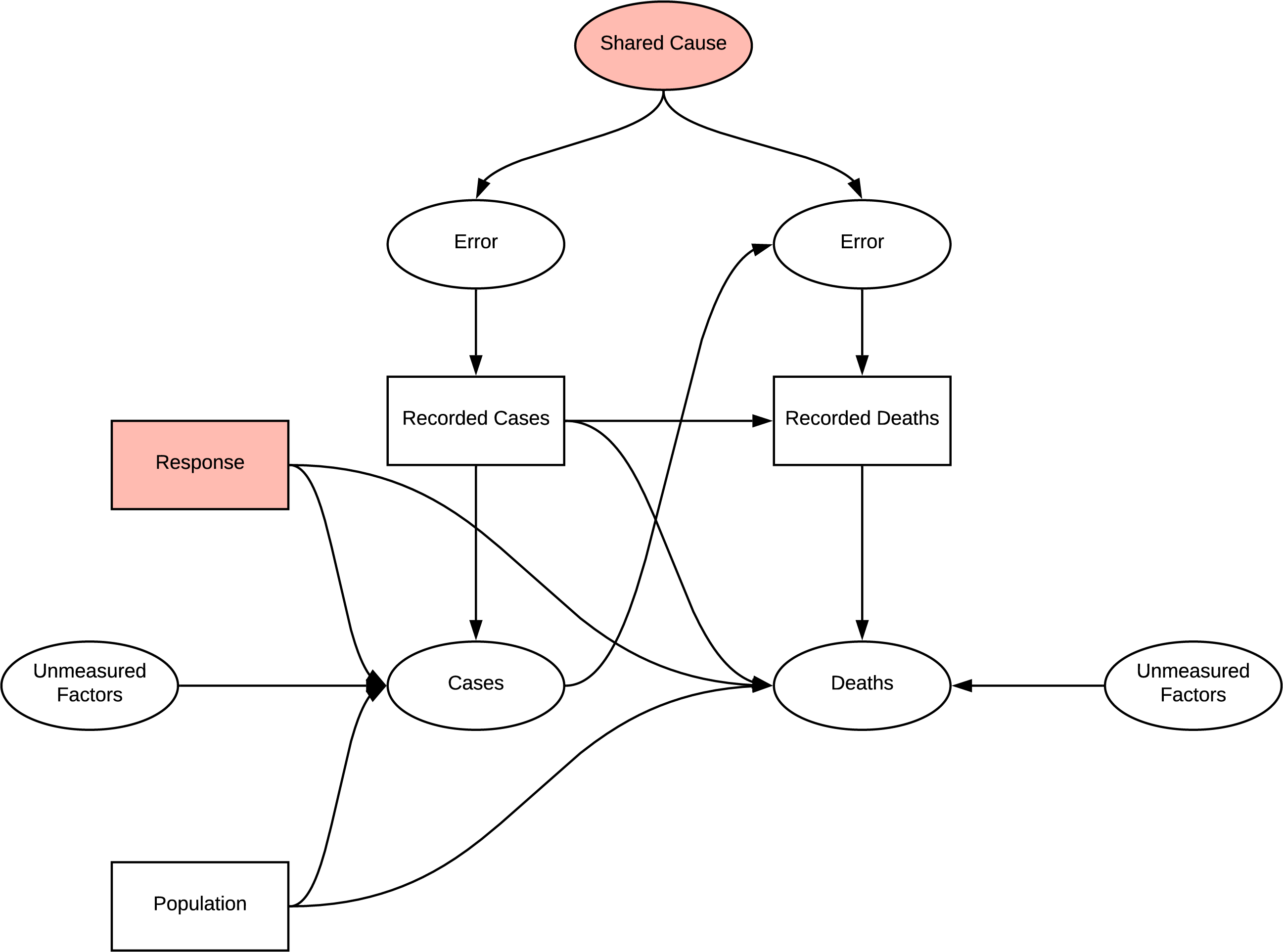
The following figure indicates the casual graph implied in the introduction of the report, the implied structure contains many sources of systematic bias. The first challenge is that the measured statistics are subject to error and do not represent the true occurrences. There are likely to be common causes of error in measuring cases and deaths due to COVID, e.g. asymptomatic patients and testing strategies. Additionally, being diagnosed with COVID is likely to influence your chance of death and weather your death will be recorded as COVID related, the bias implied by this structure is dependent differential bias (Hernán & Robins n.d.) and causes bias even under the null making it quite challenging to negate. Further, when trying to determine the effect of population on deaths there is confounding due to the common cause of response, similarly, there is confounding if any unmeasured factor affecting cases and deaths is common. There is also potential for selection bias at the collider deaths, as we would be conditioning on recorded deaths in analysis. This shows that the inferences made in the introduction should be reassessed. Further investigation of Cusal DAGs is available in Appendix B
DAG
Country Based Age Influence
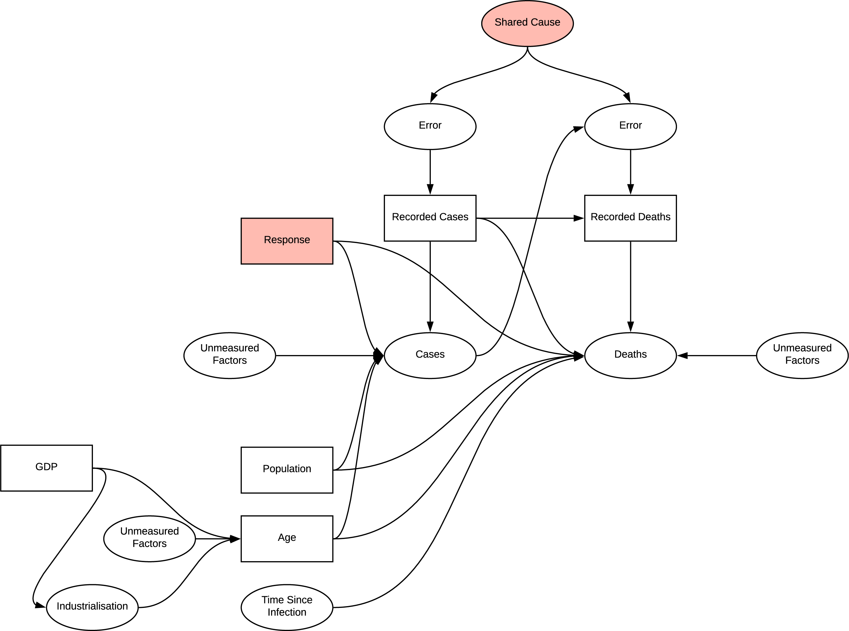
When investigating the effect of age on deaths, conditioning age on higher values opens the path to other unmeasured effects on age identified. Previously identified measurement bias is consistent in these analyses. Applying certain regression methods to age is a viable method of reducing the effect of confounding due to common cause of age, however the measurement bias is still present.
DAG
Patient Case Based Analysis
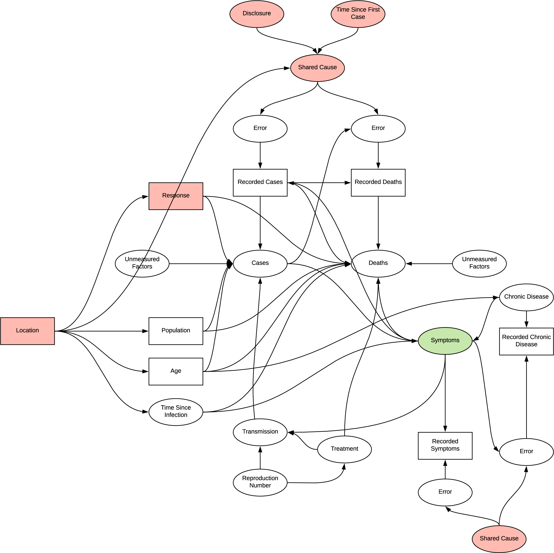
The issue with continually building on prior inferences without a framework for evaluating their structure becomes more evident here. In verifying the reason for using this dataset we instead identify two potential shared causes for measurement error; disclosure and time since first case. Additionally, as this research in focused on patient data, the location variable is introduced, a common cause of many of the observations and therefore likely to confound any analysis. It is identified that we can condition on this variable for example selecting only patient from the USA, which would potentially reduce confounding at the risk of introducing selection bias, and observe changes in distributions, however the research did not utilise this in regression. The directionality of the graph becomes quite complex with the introduction of chronic disease, introducing another source of differential dependent error. In determining if there is a connection between chronic disease and particular symptoms, conditioning symptoms opens the collider inducing selection bias, age appears to act as an additional confounder.
DAG
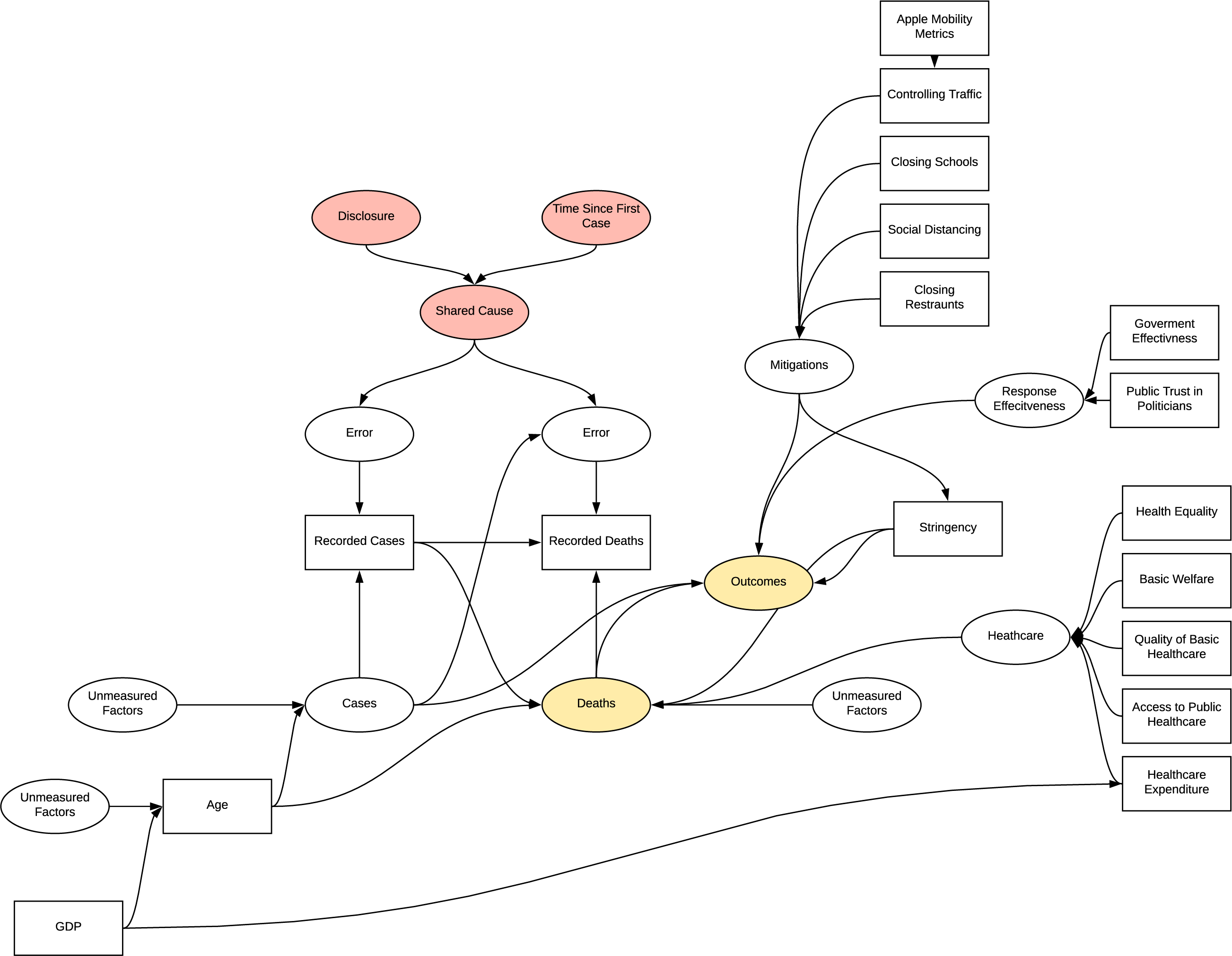
Factors and Effectiveness
All the factor analyses introduce selection biases as they select for varying conditions of outcome variables or deaths, in addition to the other bias’s observed previously. The chosen observed variables are also likely to be associated with other parts of the DAG acting as common cause confounders.
DAG
Time Varying Treatment
In both the patient based and response investigations, time varying treatment bias is introduced into the model, the complexity in displaying this prevents visualisation. In patient based investigation, the bias is due to the effect of the change in quality of treatment as understanding of the virus improved effecting the symptoms and observed. In the response investigations, as the response effects both cases and future response we see a similar effect.
Full Implied Structure
The implied structure by the research is quite flawed and has many inherent sources of systematic bias in the experiments undertaken which were not accounted for. The structure is complex developed as the research progressed, further detailing of bias in this model is unlikely to be beneficial.
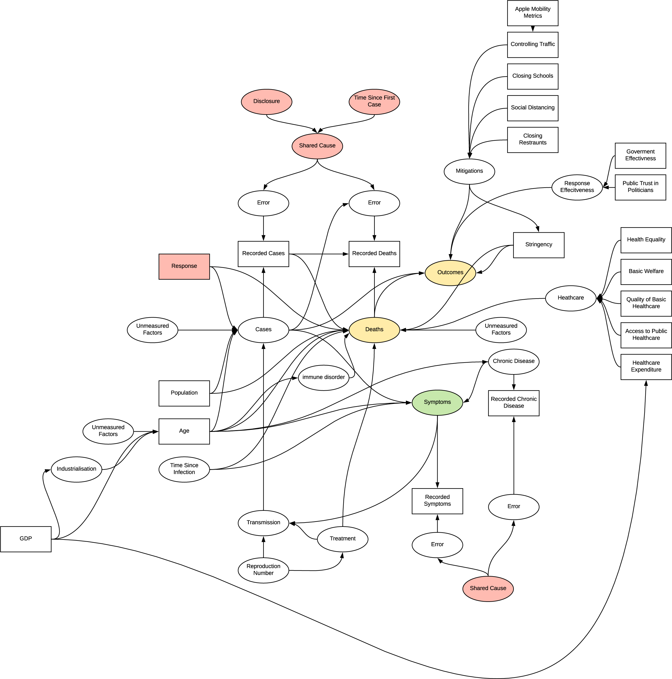
DAG